Altermagnetic Hubbard Model Example
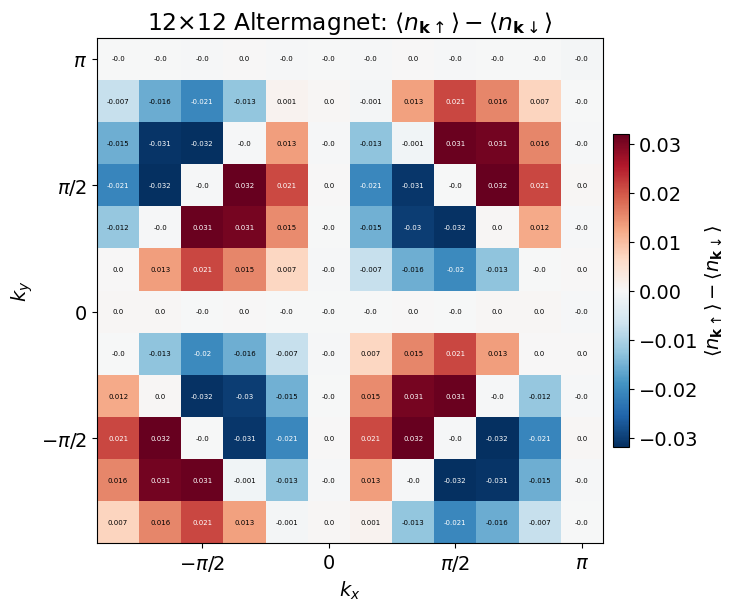
This page covers a \(12 \times 12\) altermagnetic Hubbard-model workflow followed by momentum-distribution measurement, following the model setup in Phys. Rev. Lett. 132, 263402. The reusable script remains under docs/examples/alter/, but the full commands are expanded below. In this workflow, the optimized ansatz can exhibit spontaneous symmetry breaking, which is visible in spin-resolved observables such as the momentum distribution.
12x12 PBC altermagnetic Hubbard model: momentum distribution
The altermagnetic Hubbard-model workflow uses a sublattice- and direction-dependent next-nearest-neighbor hopping. Let \(A\) and \(B\) denote the two sublattices and let \(\boldsymbol\delta_+=(1,1)\) and \(\boldsymbol\delta_-=(1,-1)\). The Hamiltonian is
Equivalently, in the \((1,1)\) direction the next-nearest-neighbor hopping element is \(t_-\) on the \(A\) sublattice and \(t_+\) on the \(B\) sublattice, while in the \((1,-1)\) direction it is \(t_+\) on the \(A\) sublattice and \(t_-\) on the \(B\) sublattice. The runs below use \(t_+=0.4\) and \(t_-=0\).
After training, the final command measures the fermionic one-body density matrix and momentum distribution,
Stage 1: determinant pretraining at U=3
python main.py \
    --output outputs/alter/12_12_N144_U8_pbc/tensor_U3 \
    --L1 12 \
    --L2 12 \
    --particles 144 \
    --U 3 \
    --t2 0.4 \
    --model hubbard_alter \
    --steps 5000 \
    --network_name tensor \
    --boundary1 pbc \
    --boundary2 pbc \
    --save_frequency 5000 \
    --use_x64 \
    --mcmc_step 360 \
    --mode adam \
    --lr 5e-2 \
    --ndet 1 \
    --reduce 500 \
    --seed 100 \
    --batchsize 4096 \
    --fast_update
Stage 2: ACE optimization at U=8
python main.py \
    --restore outputs/alter/12_12_N144_U8_pbc/tensor_U3 \
    --restore_ndet 1 \
    --output outputs/alter/12_12_N144_U8_pbc/ace \
    --L1 12 \
    --L2 12 \
    --particles 144 \
    --U 8 \
    --t2 0.4 \
    --model hubbard_alter \
    --steps 50000 \
    --network_name ace \
    --boundary1 pbc \
    --boundary2 pbc \
    --save_frequency 5000 \
    --use_x64 \
    --mcmc_step 360 \
    --mode march \
    --norm 1e-1 \
    --lr_start 1000 \
    --lr0 4000 \
    --ndet 1 \
    --hidden 144 \
    --layers 16 \
    --reduce 500 \
    --seed 100 \
    --precision tf32 \
    --batchsize 4096
Stage 3: measure the momentum distribution
python main.py \
    --output outputs/alter/12_12_N144_U8_pbc/ace \
    --L1 12 \
    --L2 12 \
    --particles 144 \
    --U 8 \
    --t2 0.4 \
    --model hubbard_alter \
    --steps 5000 \
    --network_name ace \
    --boundary1 pbc \
    --boundary2 pbc \
    --use_x64 \
    --mcmc_step 200 \
    --mode test \
    --obs fermi \
    --ndet 1 \
    --hidden 144 \
    --layers 16 \
    --reduce 2000 \
    --seed 100 \
    --precision tf32 \
    --batchsize 4096
References
- Phys. Rev. Lett. 132, 263402 — reference for the altermagnetic Hubbard-model setup.