Time Evolution with tVMC

This page expands the time-dependent VMC example. The script remains at docs/examples/tvmc/hof_8x6_obc.sh; the full commands are shown below.

Physics target

Time-dependent VMC projects dynamics onto the tangent space of the variational manifold. For parameters \(\theta(t)\) and wavefunction \(|\psi_{\theta(t)}\rangle\), the real-time TDVP update can be written as the least-squares projection

\[ \dot{\theta} = \operatorname*{arg\,min}_{v} \left\| \sum_a v_a |\partial_a\psi_\theta\rangle + \mathrm{i}H|\psi_\theta\rangle \right\|^2, \]

which gives the projected linear system \(\sum_b S_{ab}\dot{\theta}_b=-\mathrm{i}F_a\). Using the log-derivatives

\[ O_a(x)=\partial_a \log \psi_\theta(x), \]

the TDVP matrix and force can be written as covariance estimates over Monte Carlo samples:

\[ S_{ab}=\langle O_a^* O_b\rangle-\langle O_a^*\rangle\langle O_b\rangle, \qquad F_a=\langle O_a^* E_{\mathrm{loc}}\rangle-\langle O_a^*\rangle\langle E_{\mathrm{loc}}\rangle. \]

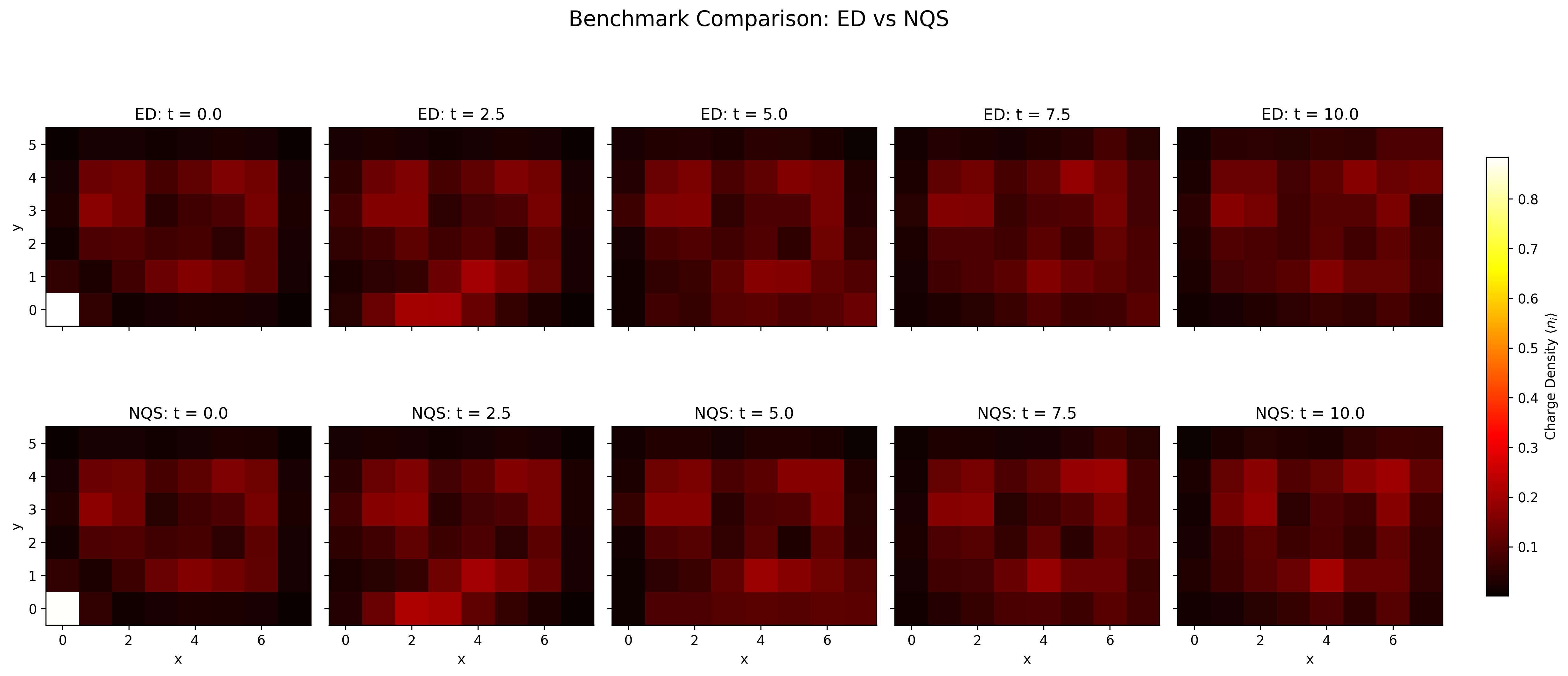
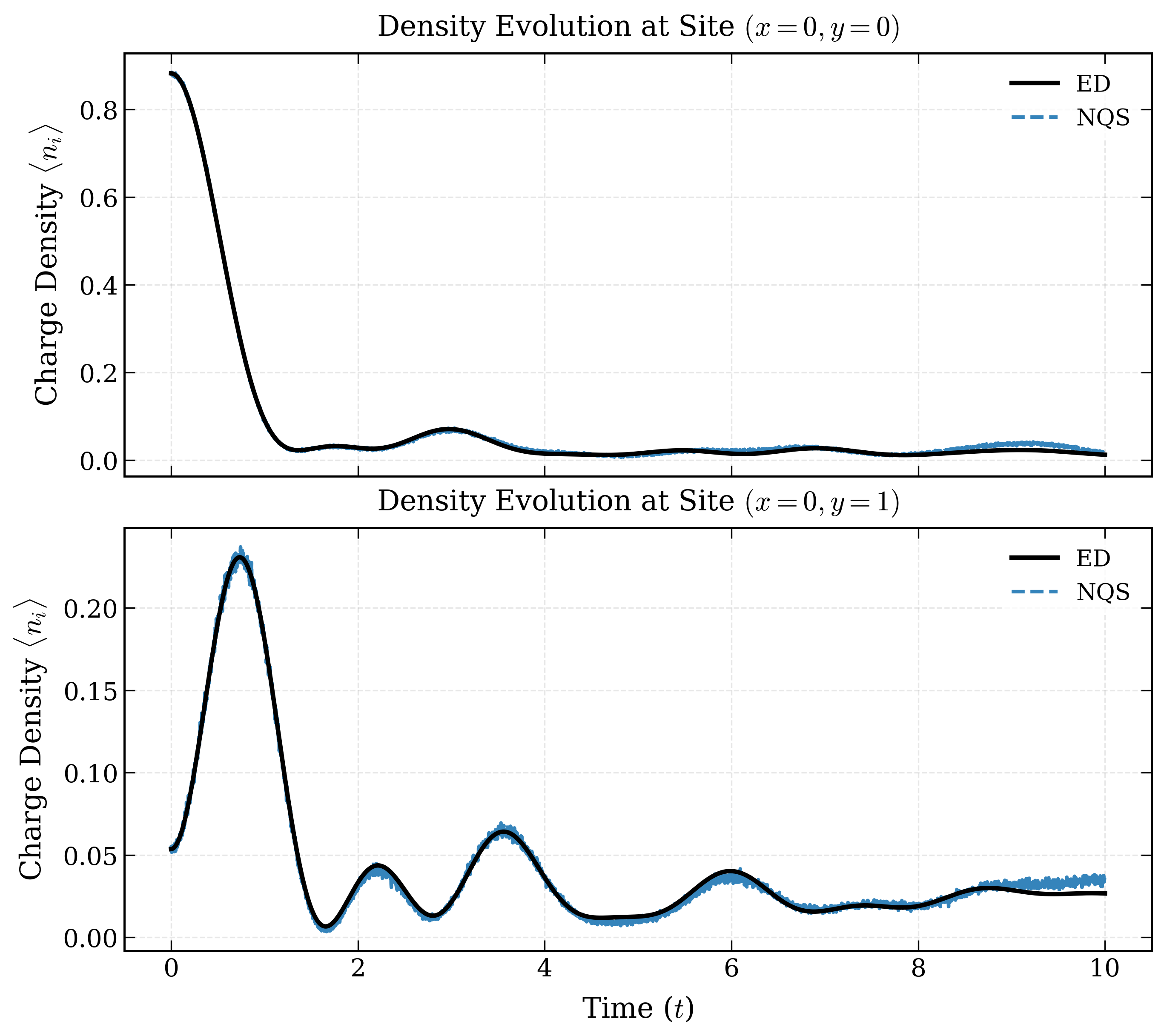
The example first trains an ACE reference state for the Hofstadter model on an \(8\times6\) open-boundary lattice. It then restores that checkpoint and uses ace_peft for parameter-efficient tVMC evolution. The ace_peft wrapper freezes the majority of the restored ACE parameters and evolves only a compact PEFT output block, following the parameter-efficient adaptation strategy in arXiv:2606.05850. This helps maintain numerical stability during time evolution.

Hamiltonian

The tVMC example uses the same interacting Hofstadter Hamiltonian as the charge-pumping Hofstadter example. During the initial training stage, --hv -4 adds a site-local pinning potential

\[ H_{\mathrm{pin}} = h_v n_0, \]

with \(h_v=-4\).

The time-evolution stage measures density with --obs density, corresponding to observables of the form

\[ \langle n_r(t)\rangle = \langle \psi_{\theta(t)}|n_r|\psi_{\theta(t)}\rangle . \]

Stage 1: train the ACE initial state

python main.py \
    --output outputs/hofstadter/8_6_N4_obc_V2/ace_small2_hv-4_N5e-1 \
    --L1 8 \
    --L2 6 \
    --particles 4 \
    --particles_up 4 \
    --V 2 \
    --alpha 0.25 \
    --hv -4 \
    --model hofstadter \
    --dtype complex \
    --steps 10000 \
    --network_name ace \
    --boundary1 obc \
    --boundary2 obc \
    --save_frequency 2000 \
    --use_x64 \
    --mcmc_step 40 \
    --mode march \
    --norm 5e-1 \
    --lr_start 1000 \
    --lr0 4000 \
    --ndet 1 \
    --hidden 128 \
    --layers 12 \
    --MLP_hidden 256 \
    --MLP_layers 1 \
    --reduce 100 \
    --pad 5 \
    --seed 100 \
    --precision tf32 \
    --batchsize 4096 \
    --polarized

Stage 2: PEFT tVMC evolution

The tVMC command restores the ACE checkpoint, switches to ace_peft, performs a burn-in, and integrates the projected equations with the Runge-Kutta Method. Because most ACE parameters are frozen, the TDVP solve acts on a smaller parameter subspace, reducing instability from over-flexible updates.

python main.py \
    --restore outputs/hofstadter/8_6_N4_obc_V2/ace_small2_hv-4_N5e-1 \
    --output outputs/hofstadter/8_6_N4_obc_V2/ace_small2_peft_tvmc_lr2e-3_rk4_B40960_svd1e-8 \
    --L1 8 \
    --L2 6 \
    --particles 4 \
    --particles_up 4 \
    --V 2 \
    --alpha 0.25 \
    --model hofstadter \
    --dtype complex \
    --steps 5000 \
    --network_name ace_peft \
    --boundary1 obc \
    --boundary2 obc \
    --save_frequency 1000 \
    --use_x64 \
    --mcmc_step 30 \
    --burn_in \
    --drop_step 200 \
    --mode tvmc \
    --lr 2e-3 \
    --integrator rk4 \
    --mu 0 \
    --solver svd \
    --pinv_cutoff 1e-8 \
    --ndet 1 \
    --hidden 128 \
    --layers 12 \
    --MLP_hidden 256 \
    --MLP_layers 1 \
    --reduce 100 \
    --pad 5 \
    --seed 100 \
    --precision tf32 \
    --batchsize 40960 \
    --polarized \
    --obs density

References

• arXiv:2606.05850 — reference for the ace_peft parameter-efficient adaptation used by this tVMC workflow.